


 06.43
06.43
 Unknown
Ideal versus standard PID form

The form of the PID controller most often encountered in industry, and the one most relevant to tuning algorithms is the standard form. In this form the  gain is applied to the
  , and
, and  terms, yielding:
gain is applied to the , and terms, yielding:
where
 is the integral time
 is the derivative time
In this standard form, the parameters have a clear physical meaning.
In particular, the inner summation produces a new single error value
which is compensated for future and past errors. The addition of the
proportional and derivative components effectively predicts the error
value at
seconds (or samples) in the future, assuming that the loop control
remains unchanged. The integral component adjusts the error value to
compensate for the sum of all past errors, with the intention of
completely eliminating them in seconds (or samples). The resulting compensated single error value is scaled by the single gain .
seconds (or samples) in the future, assuming that the loop control
remains unchanged. The integral component adjusts the error value to
compensate for the sum of all past errors, with the intention of
completely eliminating them in seconds (or samples). The resulting compensated single error value is scaled by the single gain .
In the ideal parallel form, shown in the controller theory section

the gain parameters are related to the parameters of the standard form through  and
and  .
This parallel form, where the parameters are treated as simple gains,
is the most general and flexible form. However, it is also the form
where the parameters have the least physical interpretation and is
generally reserved for theoretical treatment of the PID controller. The
standard form, despite being slightly more complex mathematically, is
more common in industry.
.
This parallel form, where the parameters are treated as simple gains,
is the most general and flexible form. However, it is also the form
where the parameters have the least physical interpretation and is
generally reserved for theoretical treatment of the PID controller. The
standard form, despite being slightly more complex mathematically, is
more common in industry.
and .
This parallel form, where the parameters are treated as simple gains,
is the most general and flexible form. However, it is also the form
where the parameters have the least physical interpretation and is
generally reserved for theoretical treatment of the PID controller. The
standard form, despite being slightly more complex mathematically, is
more common in industry.Reciprocal gain
In many cases, the manipulated variable output by the PID controller
is a dimensionless fraction between 0 and 100% of some maximum possible
value, and the translation into real units (such as pumping rate or
watts of heater power) is outside the PID controller. The process
variable, however, is in dimensioned units such as temperature. It is
common in this case to express the gain not as "output per degree", but rather in the form of a temperature  which is "degrees per full output". This is the range over which the output changes from 0 to 1 (0% to 100%).
not as "output per degree", but rather in the form of a temperature which is "degrees per full output". This is the range over which the output changes from 0 to 1 (0% to 100%).Basing derivative action on PV
In most commercial control systems, derivative action is based on PV
rather than error. This is because the digitized version of the
algorithm produces a large unwanted spike when the SP is changed. If the
SP is constant then changes in PV will be the same as changes in error.
Therefore this modification makes no difference to the way the
controller responds to process disturbances.

Basing proportional action on PV
Most commercial control systems offer the option of also basing the
proportional action on PV. This means that only the integral action
responds to changes in SP. The modification to the algorithm does not
affect the way the controller responds to process disturbances. The
change to proportional action on PV eliminates the instant and possibly
very large change in output on a fast change in SP. Depending on the
process and tuning this may be beneficial to the response to a SP step.

Sometimes it is useful to write the PID regulator in Laplace transform form:

Having the PID controller written in Laplace form and having the transfer function of the controlled system makes it easy to determine the closed-loop transfer function of the system.
PID pole zero cancellation
The PID equation can be written in this form:

When this form is used it is easy to determine the closed loop transfer function.
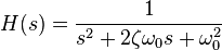
If


Then

While this appears to be very useful to remove unstable poles, it is
in reality not the case. The closed loop transfer function from
disturbance to output still contains the unstable poles.
Series/interacting form
Another representation of the PID controller is the series, or interacting form

where the parameters are related to the parameters of the standard form through
 ,
,  , and
, and
with
 .
.
This form essentially consists of a PD and PI controller in series,
and it made early (analog) controllers easier to build. When the
controllers later became digital, many kept using the interacting form.
Discrete implementation
The analysis for designing a digital implementation of a PID controller in a microcontroller (MCU) or FPGA device requires the standard form of the PID controller to be discretized.[25] Approximations for first-order derivatives are made by backward finite differences. The integral term is discretised, with a sampling time  ,as follows,
,as follows,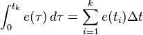
The derivative term is approximated as,
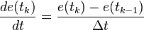
Thus, a velocity algorithm for implementation of the discretized PID controller in a MCU is obtained by differentiating  , using the numerical definitions of the first and second derivative and solving for
  and finally obtaining:
, using the numerical definitions of the first and second derivative and solving for and finally obtaining:![u(t_k)=u(t_{k-1})+K_p\left[\left(1+\dfrac{\Delta t}{T_i}+\dfrac{T_d}{\Delta t}\right)e(t_k)+\left(-1-\dfrac{2T_d}{\Delta t}\right)e(t_{k-1})+\dfrac{T_d}{\Delta t}e(t_{k-2})\right]](https://upload.wikimedia.org/math/a/9/b/a9beb5ee392aa86e76d734e9e761b148.png)


 ) and added to the controller output.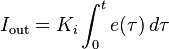



 : Derivative gain, a tuning parameter
 : Error
 : Time or instantaneous time (the present)
 : Variable of integration; takes on values from time 0 to the present
 : complex number frequency


